Bayes Classifier example

Prepare a simulated dataset for a Bayes Classifier

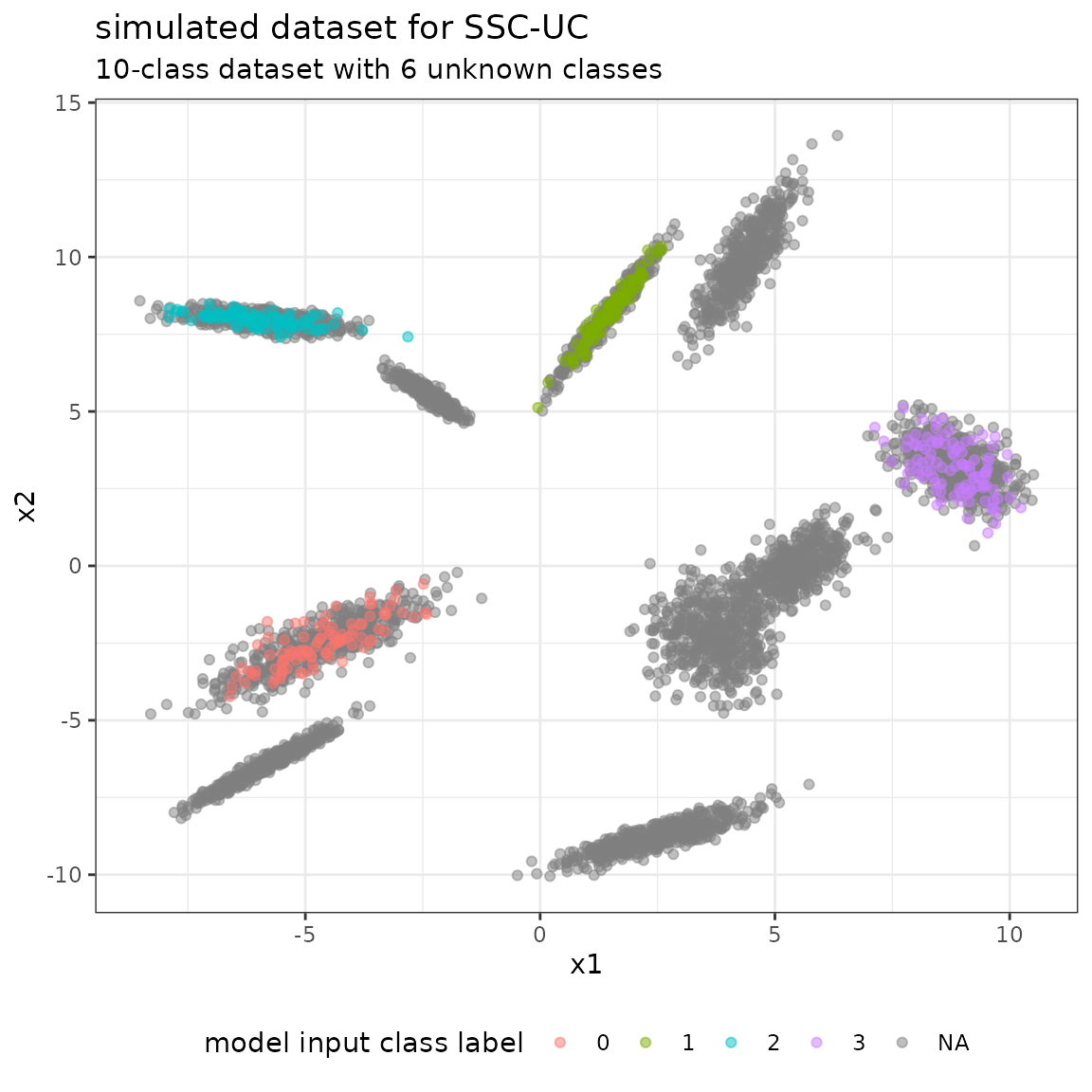
In the first step, we simulate a dataset with the following specifications:

• a total number of 10 classes, 4 of which are known and 6 are unknown, respectively
• n_labeled = 200 labeled samples, evenly distributed over the 4 known classes
• n_unlabeled = 5000 unlabeled samples, evenly distributed over the 10 classes
• a dimension of n_feats = 2 features (to facilitate representation)

Each class \(i\) is represented by a bivariate Gaussian distribution with mean vector \(\mu = (\mu_1^{(i)}, \mu_2^{(i)})\) and symmetric covariance matrix \[\Sigma_i = \left(\begin{array}{cc}\sigma_{1,1}^{(i)} & \sigma_{1,2}^{(i)} \\ \sigma_{1,2}^{(i)} & \sigma_{2,2}^{(i)}\end{array}\right).\] The known classes are 0-3.

library(mvtnorm)
set.seed(1)

# sample sizes
n_labeled <- 400
n_unlabeled <- 5000
n_feats <- 2

# mean values and covariance matrices
mu <- t(replicate(
  10,
  runif(2, -10, 10)
))
sigma <- t(replicate(
  10,
  {
    A = matrix(runif(2^2)*2-1, ncol=2)
    return(as.vector( t(A) %*% A))
  }
))
rownames(mu) <- rownames(sigma) <- 0:9

print(mu)
#>        [,1]        [,2]
#> 0 -4.689827 -2.55752201
#> 1  1.457067  8.16415580
#> 2 -5.966361  7.96779370
#> 3  8.893505  3.21595585
#> 4  2.582281 -8.76427459
#> 5 -5.880509 -6.46886495
#> 6  3.740457 -2.31792564
#> 7  5.396828 -0.04601516
#> 8  4.352370  9.83812190
#> 9 -2.399296  5.54890443
print(sigma)
#>        [,1]        [,2]        [,3]      [,4]
#> 0 1.0873223  0.69488058  0.69488058 0.6528557
#> 1 0.2686249  0.50666811  0.50666811 1.0024862
#> 2 0.6486391 -0.09008240 -0.09008240 0.0409379
#> 3 0.3940044 -0.21990520 -0.21990520 0.5422173
#> 4 0.9611412  0.40244041  0.40244041 0.2316753
#> 5 0.4985329  0.39442301  0.39442301 0.3314552
#> 6 0.3384411 -0.08302008 -0.08302008 0.9109265
#> 7 0.3644605  0.25766878  0.25766878 0.5238927
#> 8 0.2758416  0.51517414  0.51517414 1.3789753
#> 9 0.1364133 -0.12600427 -0.12600427 0.1397050

Given the data specifications, we simulate from the bivariate Gaussian distribution to generate the dataset given the class vector. We discriminate between the true class vector y_true containing the labels 0-9 of all samples, and the model input class vector y containing a true label only for the labeled data, and NA, otherwise.

# specify number of labeles / unlabeled samples per class
labeled_classes <- rep(0:3, each = n_labeled / 4)
unlabeled_classes <- rep(0:9, each = n_unlabeled / 10)
num_sample <- c(table(labeled_classes), table(unlabeled_classes))

# simulate X, ytrue and y
X <- c()
for(i in 1:length(num_sample)){
  X <- rbind(X, rmvnorm(num_sample[i], 
                  mu[names(num_sample)[i],], 
                  matrix(sigma[names(num_sample)[i],], nrow = 2, ncol = 2)
                )
             )
}
y <- rep(c(0:3, NA), c(table(labeled_classes), length(unlabeled_classes)))
ytrue <- rep(names(num_sample), num_sample)
colnames(X) <- paste0("x", 1:2)

# summaries of the model input class vector y, and the true class vector ytrue
summary(as.factor(y))
#>    0    1    2    3 NA's 
#>  100  100  100  100 5000
summary(as.factor(ytrue))
#>   0   1   2   3   4   5   6   7   8   9 
#> 600 600 600 600 500 500 500 500 500 500

Using the model input class vector y and the simulated feature matrix X, we generate the input dataset and the formula for the model.

# input dataset for the model
data <- as.data.frame(cbind(X, y))

# model formula
formula <- y ~ x1 + x2 - 1

# simulated data
head(data)
#>          x1        x2 y
#> 1 -3.438659 -2.052945 0
#> 2 -4.343196 -2.430395 0
#> 3 -6.177755 -3.426197 0
#> 4 -5.090663 -2.765295 0
#> 5 -3.318454 -1.566550 0
#> 6 -4.953884 -2.801539 0

The simulated dataset is given by the following scatterplot:

Train SSC-UC model

The SSC-UC model is called via SSCUC and returns a BayesClassifier object with known and unknown classes. In this case, a Bayes classifier is used, specified by the argument naive=TRUE.

library(SSCUC)

# train model
model <- SSC(formula, data, naive = FALSE)
#> Warning in summary.mclustBIC(BIC, data, G = G, modelNames = modelNames): best
#> model occurs at the min or max of number of components considered!
#> Warning in Mclust(X[newclass_inds, !const_cols, drop = F], G = g_opts,
#> modelNames = gmmModelName, : optimal number of clusters occurs at max choice
#> [1] "Starting EM with 6 classes"
#> Warning in BayesClassifier(formula, data, naive = naive, prior = prior, :
#> BayesClassifier removed 1957 NAs
#> [1] "EM converged after 5 iterations"
#> [1] "BIC: 18418.8851091367"
#> [1] "Trying EM with 5 classes"
#> Warning in BayesClassifier(formula, data, naive = naive, prior = prior, :
#> BayesClassifier removed 1957 NAs
#> [1] "EM converged after 4 iterations"
#> [1] "BIC: 22778.8389840301"
#> [1] "BIC increased when updating - stopping"
summary(model)
#> BayesClassifier model with 10 classes and 2 non-constant features
#> ==============================
#> formula:  y ~ x1 + x2 - 1 
#> used features:  x1, x2 
#> parameters:

	mu	Sigma	prior
0	-4.66,-2.53	0.84,0.52,0.52,0.5	0.09
1	1.47,8.19	0.27,0.48,0.48,0.96	0.11
2	-5.94,7.96	0.67,-0.09,-0.09,0.05	0.11
3	8.81,3.25	0.31,-0.18,-0.18,0.44	0.09
U1	2.51,-8.77	0.96,0.4,0.4,0.24	0.09
U2	4.55,-1.18	1.08,1.06,1.06,1.93	0.18
U3	-5.88,-6.47	0.56,0.45,0.45,0.4	0.09
U4	-2.4,5.55	0.13,-0.11,-0.11,0.13	0.09
U5	4.37,9.92	0.27,0.5,0.5,1.37	0.09
U6	0.29,1.24	43.47,11.45,11.45,17.91	0.05

Predict and evaluate unlabeled data using SSC-UC model

Class labels for the unlabeled data in the dataset are obtained using the predict function with argument type=“class”.

# predict on unlabeled data
pred <- predict(model, newdata = subset(data, is.na(y)), type = "class")

Evaluate in full confusion matrix (multiple unknown classes)

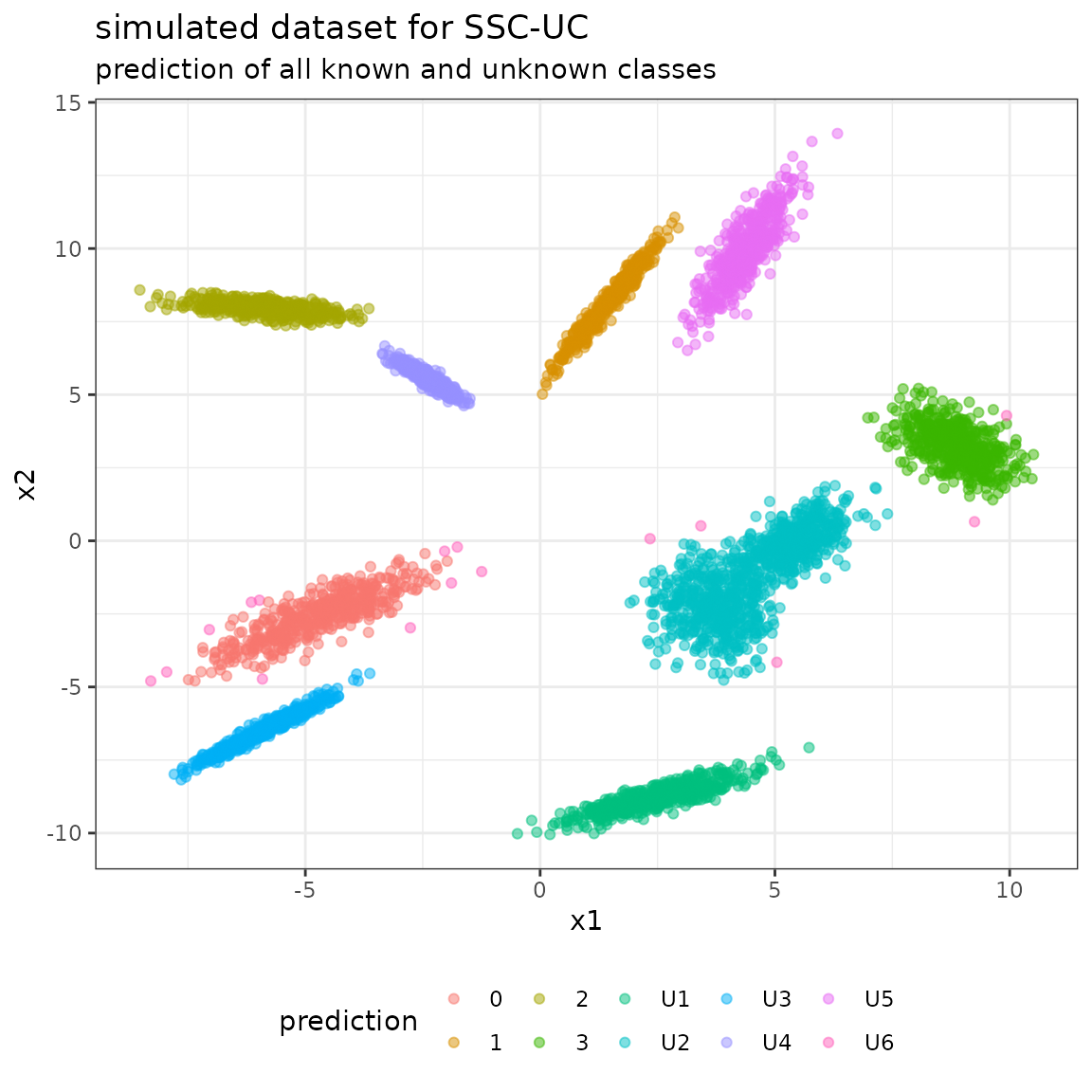
The full confusion matrix contains all the classes modeled by the BayesClassifier:

• the class labels 0-9 from the data specification as reference labels (not that, however, only classes 0-3 are known to the model a-priori),
• the class labels for known classes (0-3) and unknown classes (U1-U8) as predicted labels.

library(caret)
#> Loading required package: lattice
library(knitr)

# specify levels
levels <- sort(union(unique(pred), unique(ytrue)))

kable(confusionMatrix(
  reference = factor(ytrue[is.na(y)], levels = levels), 
  data = factor(pred, levels = levels))$table[sort(unique(pred)),sort(unique(ytrue))]
)

	0	1	2	3	4	5	6	7	8	9
0	489	0	0	0	0	0	0	0	0	0
1	0	500	0	0	0	0	0	0	0	0
2	0	0	500	0	0	0	0	0	0	0
3	0	0	0	498	0	0	0	0	0	0
U1	0	0	0	0	500	0	0	0	0	0
U2	0	0	0	0	0	0	497	500	0	0
U3	0	0	0	0	0	500	0	0	0	0
U4	0	0	0	0	0	0	0	0	0	500
U5	0	0	0	0	0	0	0	0	500	0
U6	11	0	0	2	0	0	3	0	0	0

The following plot shows the unlabeled data with their predicted class labels:

Evaluate in reduced confusion matrix (all unknown classes as class “U”)

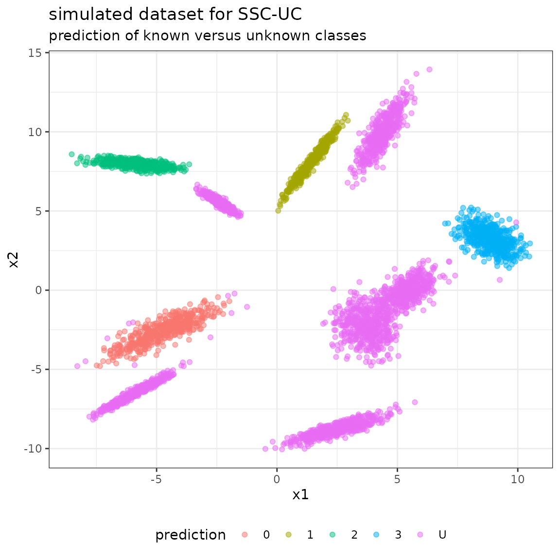
As a second evaluation step, we can summarize all “unknown” classes detected by SSC-UC into one class “U” (unknown). Thereby, we reduce the number of labels in the confusion matrix to 0-3 and U.

# set all new class labels to "U"
pred[!pred %in% unique(ytrue)] <- "U"

# specify levels
levels <- sort(union(unique(pred), unique(ytrue)))

kable(confusionMatrix(
  reference = factor(ytrue[is.na(y)], levels = levels), 
  data = factor(pred, levels = levels))$table[sort(unique(pred)),sort(unique(ytrue))]
)

	0	1	2	3	4	5	6	7	8	9
0	489	0	0	0	0	0	0	0	0	0
1	0	500	0	0	0	0	0	0	0	0
2	0	0	500	0	0	0	0	0	0	0
3	0	0	0	498	0	0	0	0	0	0
U	11	0	0	2	500	500	500	500	500	500

The following plot shows the unlabeled data with their predicted class labels, when considering all unknown classes as one class.